I’ve been asked to provide the contents of my hour long video presentation about processing of industrial IoT data streams as an article that can be read and browsed at your own pace. Well, I’m happy to oblige…

Introduction

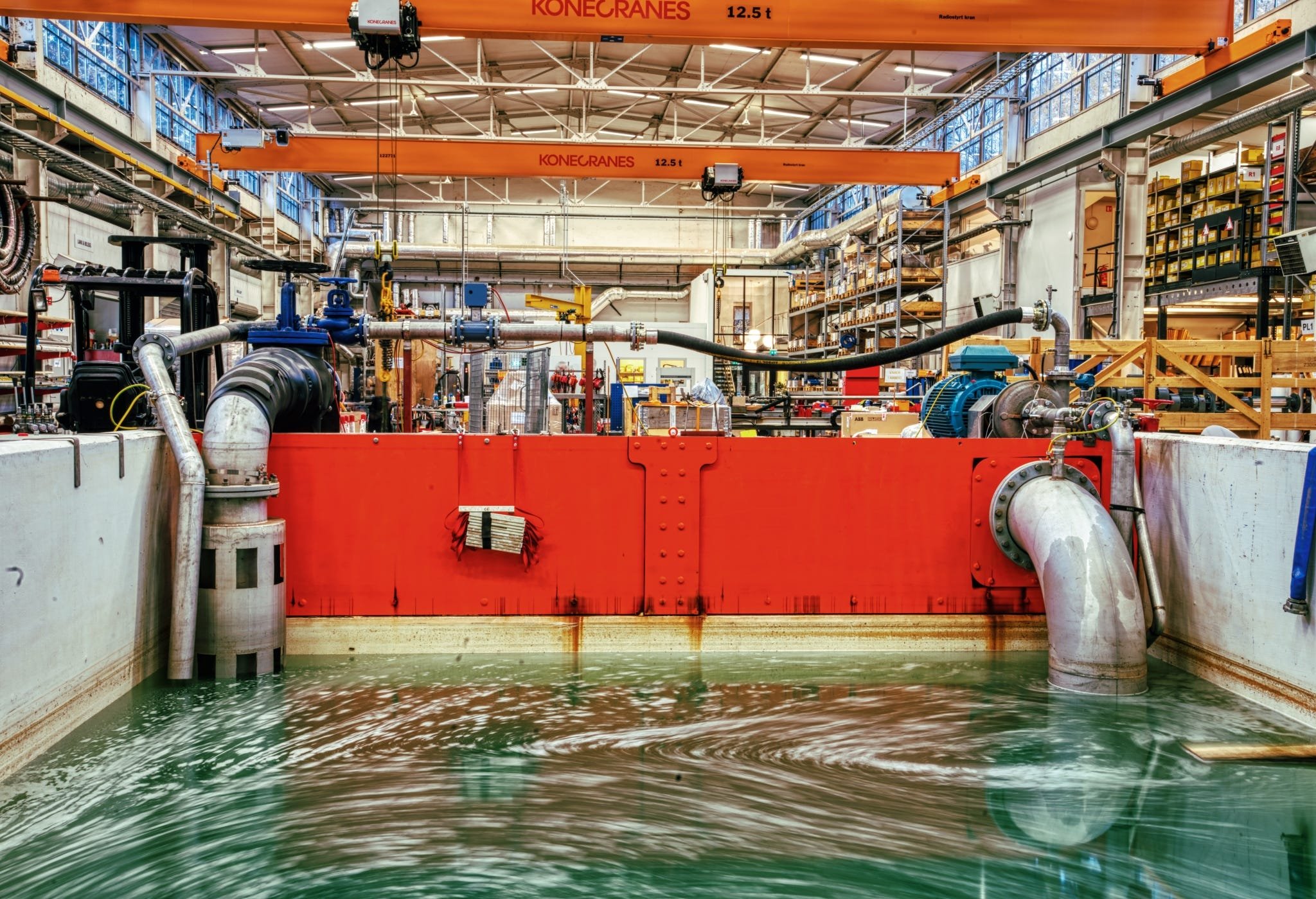
Streaming industrial IoT data can be complicated to process, because it often involves a large amount of data, received in continuous streams that never end. There’s never one single machine to monitor. Always a number of them. Multiple buildings, one or more factories, a fleet of ships, all of an operator’s subsea oil pipelines. That kind of scale.

Industrial IoT is never implemented just for fun. There needs to be real, reasonably short term, economic value involved. Alternatively it needs to be about fulfilling new environmental requirements.

 

Data sources and data rates

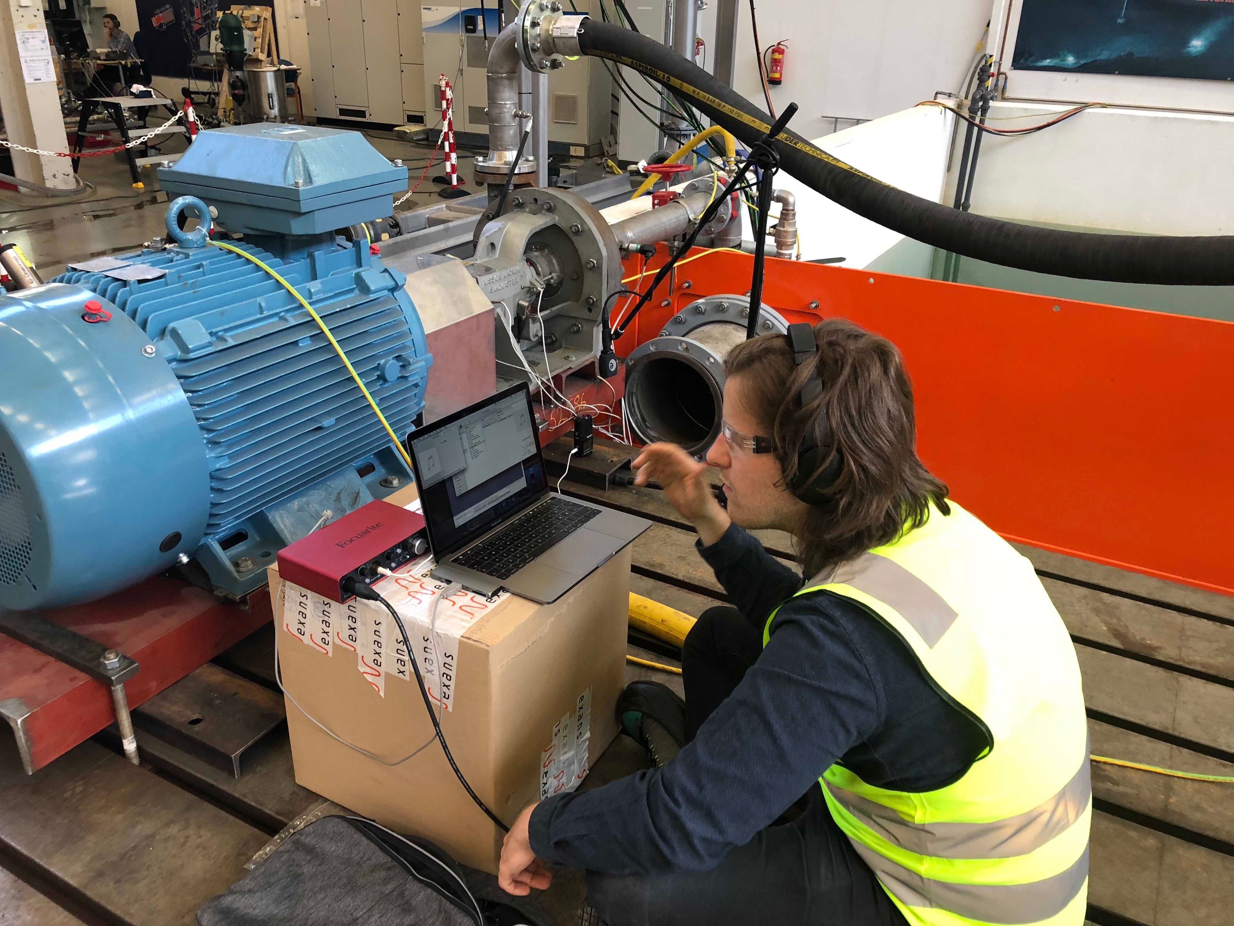
You would need a data rate of minimum one measurement per minute from multiple sensors, in order to detect the need for maintenance of pumps and generators for the oil industry. You might have to increase that to every second or so, if you’re working with engines or production equipment with higher rotational speed.

One of the storage solutions I’ve been working on is currently receiving more than 20.000 sensor measurements per hour. 500.000 values per day. From a single smart building equipped with 5400 sensors. It used to be 125.000 sensor measurements per hour, that is 3.000.000 values per day, but we tweaked the sample rates, based on customer needs and requirements. We also worked on local buffering mechanisms with micro batching. That storage mechanism is almost idling now, ready for scale out, enabling thousands of smart buildings to be connected in the near future.

A single surface mounted microphone will deliver between 40.000 and 200.000 samples per second to those who want to explore sound. By then you might have to fast fourier transform the audio, and run machine learning on the dominant frequencies and their amplitudes. A trained machine learning model could potentially run on an edge device close to the microphone, instead of in the cloud.

Also video streams are interesting, given that you’re able to separate anomalies from what’s normal, preferably before you waste lots of bandwidth.

 

Processing on edge devices

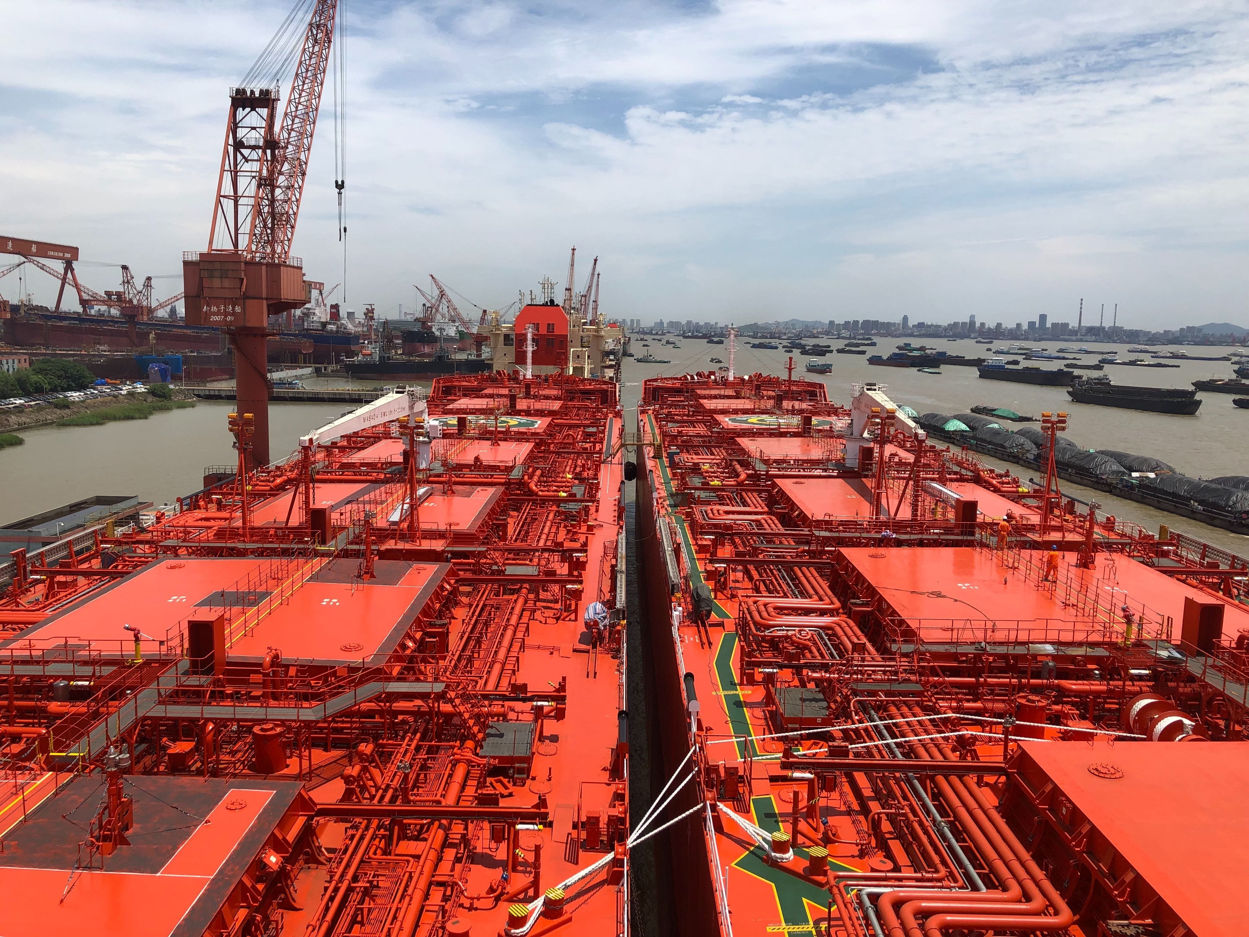
IoT data may need to be buffered for multiple weeks, if your sensors and equipment are at sea. They may need to be transferred to the cloud when the ship is in a harbour, or the data may be brought to shore on removable disks. IoT data streams don’t have to be transmitted in real time to provide value. Though, sometimes you’ll want to perform at least parts of the processing on site. For example optimization of fuel consumption for tankers and tug boats, or detection of anomalies or maintenance prediction for subsea oil pumps.

It’s perfectly possible to run trained machine learning algorithms on quite primitive equipment, like relatives of Raspberry PI, or a small rugged PC. Maybe directly on your IoT gateway, that in some cases can be as powerful as any server blade. You also won’t need a lot of machines to be able to deploy a reasonably redundant Kubernetes cluster, even if your architectural choices become much more limited than they would have been with a cloud provider.

You may actually find a local cloud, like Azure Stack, on an oil rig. But I wish you luck with getting certifications and permission to deploy your own software to one of those.

 

Trivial stream processing

Your stream processing gets really simple, if all you need to do is to call an already trained machine learning algorithm.

You provide for receiving all sensor measurements relevant to the algorithm, using sensible data rates for the purpose, and feed that to the model as the data arrives.

You may also want to store all the data as cheaply as possible in HDFS, a data lake, or in BLOB storage, in a way that makes it easy to separate both equipment and days, for the next time you require data to retrain the algorithm.

This type of data stream filtering is easy to implement using Kafka, or Azure Stream Analytics. And you can perfectly well do this in addition to other stream processing.

But most customers of industrial IoT, require something more tangible, in addition to just a callable algorithm that detects something fancy.

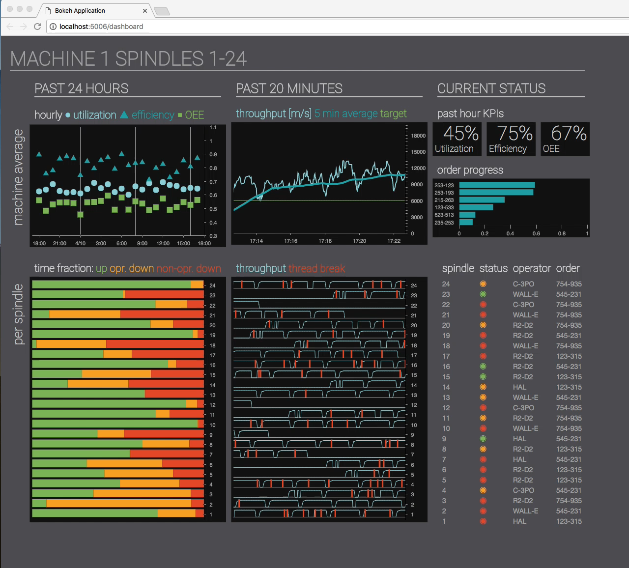
They often require dashboards that show how production does in real time, with fancy graphs, multiple dimensions, color coded performance and downtime.

These dashboards may have low practical utility beyond showing them off at board meetings, or talking about them to people you want to impress. But they can on the other hand be extremely hard to implement. Particularly when your customer also wants parameterizable reports that can compare current and historic periods of time.

The rest of this article will be about architectural choices geared towards solving these kinds of tasks.

 

Aggregation

The key to create fast updating charts and reports, is to store the underlying data on a format that can easily be combined into the desired result, with a resolution that doesn’t require too much work per recalculation. These precalculations are typically aggregations. Grafana and Plotly Dash are two very good tools to implement these kinds of user interfaces.

The aggregated precalculations must be stored somewhere. This storage space is often termed Warm Storage, because it provides high availability access to preprocessed data, with granularity suited for presentation purposes. This is opposed to cold storage, which typically stores all the data, in original form, which usually requires a certain amount of time and effort to retrieve and process before use.

If you store the count of values, the minimum value, the maximum value, the sum of values, and the sum of squares of each value, for a set of time intervals. Then you can easily calculate the average, standard deviation, variance, sum, count, minimum and maximum for any combination of the time intervals, using simple formulas. The example uses PostgreSQL / TimescaleDB syntax:

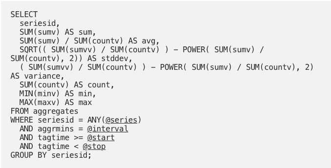
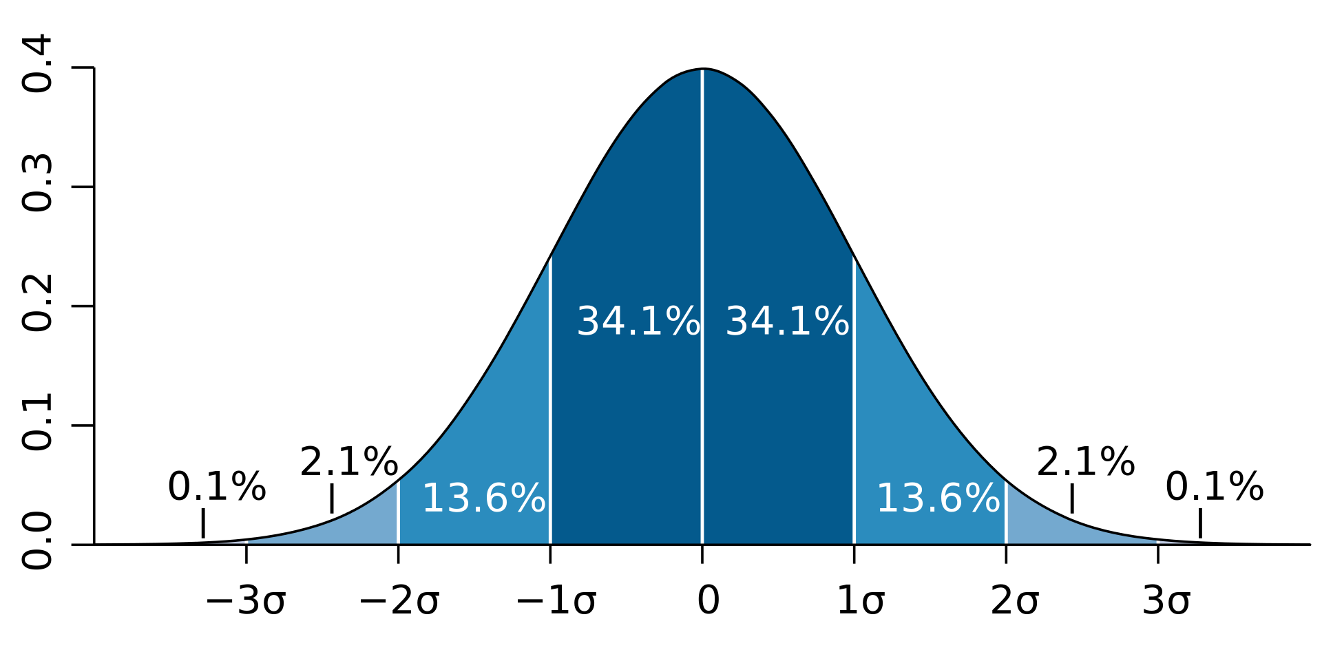
Average and standard deviation can be used to display normal distribution bell curves for values within the combined intervals. Thus the aggregates still retain quite a bit of information about the original raw values.

 

 

 

Warm storage

As a Data Scientist, you’ll often find that just observing the values that stream by doesn’t give you enough context to perform complex calculations. You may need a cache of recent data, or a place to store partial precalculations, aggregates, and potentially the output of machine learning models, typically for use in dashboards and interactive parameterized reports. I’ll call this data cache warm storage.

Warm storage is often used used by Data Science applications, and algorithms that call machine learning models, in order to quickly retrieve sufficient sensor values and state changes from streaming data. Warm Storage data may typically be used to detect anomalies, predict maintenance, generate warnings, or calculate Key Performance Indicators, that add insight and value to streaming data for customers.

Those KPIs are often aggregated to minute, ten minute, hour or day averages, and stored back into warm storage, with a longer retention period, to facilitate reuse by further calculations. The stored partial aggregates may also be used for presentation purposes, typically by dashboards, or in some cases reports with selectable parameters. Thus optimal retention periods may vary quite a bit between tenants and use cases.

Properties of a good Warm Storage

• Has a flexible way of querying for filtered sets (multiple series) of data
• Can match and filter hierarchical tag IDs in a flexible manner
• Has low latency, and is able to retrieve data quickly on demand
• Supports storage and querying of KPIs and aggregates calculated by data science algorithms, that potentially call machine learning models
• Exposes ways of building upon previously calculated data
• Contains only data that has a potential to be actively queried
• Has a Python wrapper for easy method invocation
• Behaves similarly when running on an Edge device

An often overlooked topic is that Warm Storage should be opt out by default, not opt in. Every insert into Warm Storage will cost you a little bit of performance, storage space, and memory space for indexes, before it is removed as obsolete. All data that is scanned through, as part of index scans during queries, will also cost you a little bit of io, memory and cpu, every time you run a query. Tenants that have no intention to use Warm Storage should not have their data stored there. Neither should tags that will never be retrieved from Warm Storage. The first rule of warm storage is: Don’t store data you won’t need. Excess data affects the performance of retrieving the data you want, costs more money, and brings you closer to a need for scaling out.

A good Warm Storage should have a Python wrapper, to make it easier to use from Data Science projects. If you’re using Warm Storage in a resource restricted environment, like on an edge device, the API should behave the same as in a cloud environment.

Existing stream processing products

Most of the existing stream processors, like Apache Spark, Storm and Flink, are very focused on performing MapReduce in real time on never ending data streams. That’s obviously immensely powerful, and you can do lots of interesting things to data streams that way. But, it’s overkill, and unnecessarily complicated, if all you’re looking for is some aggregations, calculations of a few Key Performance Indicators, and a bunch of simplistic alarm triggers.

The exception seems to be Kafka Streams, KSQL for Kafka, and Apache Samza. All of those let you consume Kafka topics, in order to send derived streams back into Kafka, in the shape of new topics or tables. Kafka, which primarily is sort of a cloud sized message bus on steroids, is interesting in many ways, but also quite large and complex. It actually feels a bit daunting to install, configure and use Kafka for the first time. You just know there’s a huge learning curve ahead, before you’ll be able to achieve a mature solution. Additionally, Kafka wouldn’t be my first choice to store large amounts of sensor data for a long time, even though RocksDB, the database engine for Kafka KTables is a good one. Confluent provides a managed Kafka cloud service, which works with Google Cloud, Azure, and Amazon Web Services.

Let’s keep Kafka, and particularly KSQL with KTables, in the back of our minds. In the meantime, let’s have a look at what time series databases can offer us.

InfluxDB highlights

InfluxDB is open source, and probably the fastest time series database on the market. It’s capable of running on reasonably powered edge devices. InfluxDB uses a text based format called line protocol for adding data, but has a SQL like query language.

InfluxDB utilizes a completely static data structure, centered around the timestamp, with attached value fields and metadata strings called a tag set. The metadata are indexed, and you can search using both metadata and time ranges within each time series.

InfluxDB doesn’t support updates, but you can delete specific data between two timestamps, or drop an entire time series. You can also overwrite the value fields, if you take care to use exactly the same timestamp and tag set. That’s usually almost as good as being able to update.

InfluxDB performance is closely coupled to cardinality, which is all about how many metadata tags that need to be indexed, and that are scanned during queries. All queries must be bounded within a time range, to avoid performance crises. InfluxDB supports automatic aggregation and calculation of derived values, by means of so called continuous queries. Deletion of old data can be handled automatically by retention policies. Both of these mechanisms cost a little bit of performance when they are used.

InfluxData have implemented their own database engine, written in Go. What scares me a bit, is the number of stories on support forums, about people who wonder how they lost their InfluxDB data. There is a managed InfluxDB service available on cloud.influxdata.com.

TimescaleDB highlights

TimescaleDB is an extension to the PostgreSQL relational database. Both are open source. TimescaleDB splits tables into partitions called chunks, based on a predefined time interval, or automatically, as time series data are written to each hyper table. These chunks are really tables themselves, and have individual indexes. Only a few of these smaller indexes need to stay in memory most of the time. This as good as eliminates the major problem with utilizing relational databases for time series data, provided that all your queries confine themselves to reading from a low number of chunks, and that each chunk contains no more than 25 to 50 million rows.

Queries, inserts, updates and deletes across chunks are handled transparently, with standard PostgreSQL syntax. Dropping entire chunks at a time is a very effective way of implementing retention limits, to get rid of expired data.

It’s necessary to use connection pooling, if you want to use TimescaleDB from a REST API. You also need to control the connection timeout and the statement timeouts. You can write only to the master node, when using a high availability PostgreSQL cluster like for instance Patroni, but you can scale reading, by sending queries to all the replicated slave nodes.

TimescaleDB exists as a managed service on timescale.com/cloud, and as managed PostgreSQL for Azure. You can scale both TimescaleDB and InfluxDB by sending unrelated time series data, for instance belonging to different customers, to separate database clusters. This kind of scale out is commonly called sharding.

TimescaleDB and InfluxDB could both handle long term storage and aggregate storage responsibilities in low resource environments, like when your customer doesn’t want to use cloud services, or when you want to analyze sensor data close to the relevant equipment, for connectivity or reduced latency reasons. This is commonly called edge computing or running on edge devices.

Cassandra highlights

Cassandra is a distributed cloud storage service based on Google BigTable technology. It needs to run on multiple machines, and isn’t capable of running on single node edge devices in a sensible way. Cassandra has many features that make it particularly well suited for handling time series data.

Cassandra utilizes a masterless architecture with no single point of failure, and scales almost linearly to a large number of machines, VMs or Pods, as the need for storage space grows. Data is stored compressed and redundantly, with multiple copies across several nodes. You should avoid using Cassandra on top of redundant disk volumes. That would simply increase the storage requirements, and lower the performance. Cassandra is optimized for write performance over query speed, updatability and deletes.

The query language is a lot like SQL, and supports complex data structures like lists, sets, maps, json objects, and combinations of these as column types. Cassandra is not a relational database, and doesn’t use joins. All Cassandra queries and commands should be performed asynchronously. Data that belongs together is partitioned on the same node, to improve query performance. It might be a good idea to store multiple copies of data, instead of creating secondary indexes, whenever you need to retrieve that same data using different access patterns.

On paper, hBase and OpenTSDB, a dedicated time series database built on top of hBase, seem like good alternatives to Cassandra. hBase is however more complex to configure, maintain, and code for than Cassandra. Another interesting alternative is ScyllaDB, which claims to be a self optimizing Cassandra, reimplemented in C++, in order to achieve performance gains. ScyllaDB is rather new, and doesn’t yet have the huge community support that Cassandra enjoys.

Storage strategies

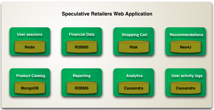
Storage is cheap. Store IoT data the way you want to read it. Feel free to store multiple copies in alternate ways. That’s called query driven design. Don’t be afraid to utilize multiple storage services for different purposes. Martin Fowler eloquently describes this as polyglot persistence.

 

Joins and transactions are as good as irrelevant for IoT data streams. They don’t change after they’ve been sent, and joins cost performance. You may also need multiple aggregation intervals for different purposes. Preferably aggregate each granularity lazily, after you’re comfortable that the underlying data have arrived, and not every single time relevant data arrives.

Utilizing mechanisms like time to live indexes, or time to live tombstoning, can affect performance surprisingly easily. Try to find a way to utilize deletion of chunks or other partitions, whenever your storage mechanism supports that. It can be very inefficient to delete expired data by searching through or recompressing huge amounts of data. Sometimes it’s far better to simply leave expired data where they are, rather than spending time and resources cleaning up. It may in some cases also give you cheaper cloud provider bills.

You can implement your own partitioning, by writing data to separate tables, depending on timestamps within predefined intervals, and then drop the oldest tables when all their data have expired. The disadvantage is that you must create and drop tables dynamically, and may need to read from more than one of the tables at a time. This could be a way to implement a short term buffer efficiently in Cassandra, which is able to handle several millions of inserts per second, when scaled out.

Native types and index sizes

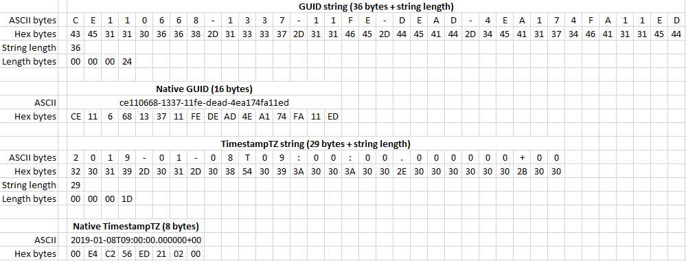
Always strive to use native database types for your index columns. Native types are often much more compact than string representations, and are scanned using pure binary comparisons. Definitely never using case insensitive or culture dependent collations, which can happen if you’re not careful about how you define string columns. A native UUID is stored in 16 bytes, and can be compared as two 64 bit integers. A UUID string is 36 bytes long, plus the length marker, and is hopefully compared in a case sensitive ordinal way. A native timestamp with time zone is stored in 8 bytes, and can be compared as one 64 bit integer.

 

This seems like a small thing, and I know we’re not supposed to pre optimize, but it’s really about the innermost of inner loops. An industrial IoT storage solution surely performs billions of index comparisons every day. The indexes are read from disk into memory cache, often called the buffer pool, where the index blocks are traversed, and hopefully remain until the next time each index block needs to be checked, unless another index block needed the same memory space more urgently. Eventually you can get buffer pool thrashing, where index blocks are read from storage into memory over and over, because the buffer pool is too small for the most frequently used index blocks.

You can expand the size of the buffer pool, until it’s constrained by the memory installed in the machine, or maybe more typically allocated to the virtual machine. But another thing that really helps is when the indexed column values are compact, and simple to compare, for every row. This maps directly to less index data to read from storage, and room for more index data in the same buffer pool. You should also strive to avoid large index range scans, by writing your queries carefully, and by storing data as you want to access it, optionally utilizing multiple copies.

Micro batching

Database systems like Cassandra support batching of commands on an API and protocol level, and can execute batches asynchronously on multiple nodes. That’s particularly effective when the entire batch uses the same partition key. But batching can be supported even using SQL, when you know the syntax. Utilize this to write multiple values using the same command, so that the number of network roundtrips is reduced. You’ll spend much less time waiting for network latency. The example uses PostgreSQL / TimescaleDB syntax:

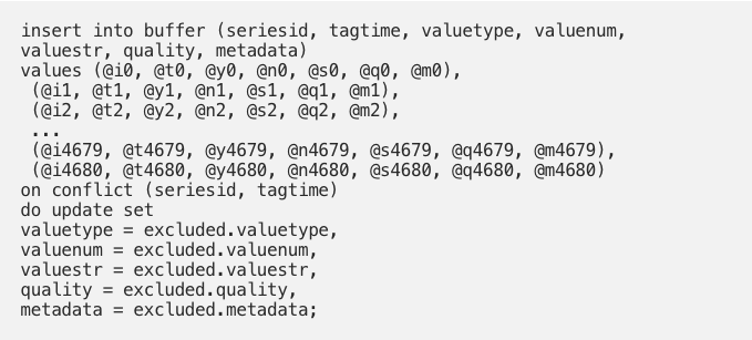
I encourage the use of arrays, when writing your own REST APIs. Use arrays actively for inserting multiple values, and for retrieving sets of series in the same method call. This makes life easier for data scientists, and reduce the aggregated network latency when using the API. Reducing latency for things you do often, improves performance.

You should strive to send and receive multiple elements per call, when you’re using queues for IoT data. Most queue implementations support this, and utilizing it can reduce the need for scale out significantly. Handling each sensor measurement typically represents very little processing. Thus you might as well receive a number of them at a time, to avoid the aggregated network latency of fetching them one by one.

Micro batching performance

Utilizing micro batching all the way through, including synchronizing sample timestamps, or buffering upstream for a few seconds, can have a profound impact on performance. I’ve seen 10.000 sample values written to the short term buffer, with a full copy to the long term storage, registering 4.000 new scheduled aggregations, and updating 12.000 statistics log entries complete in 3 seconds, as a single micro batch.

It’s likely that handling each sample value would take around 100 milliseconds, if those same 10.000 sample values were to be processed individually, on the same storage system. Some of it would definitely be handled asynchronously, but we could easily end up at around 500 seconds total. More than 8 minutes of processing time, for those same 10.000 sample values that micro batching handled in 3 seconds.

You could certainly scale out as an alternative, and process more in parallel. But scale out costs money, in the shape of larger bills from your cloud provider. Not utilizing micro batching may at one point limit the total throughput you’ll be able to achieve, and the difference between using it and not can be dramatic. Besides, you can scale out while using micro batching too.